A Comprehensive Guide to Common Supervised Learning Methods

Supervised learning is a fundamental concept in machine learning, where we teach models to learn patterns and make predictions based on labeled data. In this blog post, we'll explore the most commonly used supervised learning methods, understand how they work, and discuss their advantages and disadvantages. We'll also provide Python examples for each method and compare their performance on the popular Iris Flower dataset.

Commonly Used Supervised Learning Methods

1. Linear Regression

Overview: Linear regression is a simple, yet powerful method used for predicting a continuous target variable based on one or more input features. It finds a linear relationship between the features and the target variable.

Real-World Example: Predicting house prices based on features like square footage, number of bedrooms, and location.

How it Works: Linear regression minimizes the sum of squared errors between the predicted and actual values. It uses the equation of a straight line (y = mx + b) to make predictions.

Advantages:

• Simplicity: Linear regression is straightforward to understand and implement, making it an excellent choice for beginners.

• Interpretability: The model's coefficients can provide insights into the relationship between input features and the target variable.

Disadvantages:

• Linearity Assumption: Linear regression assumes a linear relationship between input features and the target variable, which may not hold for all datasets.

• Limited Complexity: It may not capture complex relationships in the data, limiting its predictive power.

Python example

# Import libraries
import numpy as np
import matplotlib.pyplot as plt
from sklearn.linear_model import LinearRegression
from sklearn.metrics import mean_squared_error

# Load and prepare the data
from sklearn.datasets import load_iris
iris = load_iris()
X = iris.data[:, :2]
y = iris.target

# Fit a linear regression model
model = LinearRegression()
model.fit(X, y)

# Make predictions
y_pred = model.predict(X)

# Calculate Mean Squared Error
mse = mean_squared_error(y, y_pred)
print(f"Mean Squared Error: {mse}")

Output:

Mean Squared Error: 0.18269081973947734

Script explain:

• X: This variable contains the feature matrix. In this example, we've selected only the first two features from the Iris dataset for simplicity.

• y: This variable contains the target variable, which represents the class labels in the Iris dataset.

• model: LinearRegression class from scikit-learn.

• model.fit(X, y): This method fits the linear regression model to the training data (X and y), estimating the coefficients of the linear equation.

• y_pred: This variable holds the predictions made by the linear regression model on the input data X.

• mse: This variable stores the Mean Squared Error, which measures the average squared difference between the actual and predicted values.

2. Decision Trees

Overview: Decision trees are versatile algorithms used for both regression and classification tasks. They create a tree-like structure to make decisions based on input features.

Real-World Example: Classifying whether an email is spam or not based on its content.

How it Works: Decision trees recursively split the data into subsets by selecting the most informative features at each node. The leaves of the tree contain the predicted values or classes.

Advantages:

• Easy to Understand: Decision trees are intuitive and can be visualized, making them great for beginners.

• Can Handle Mixed Data Types: Decision trees can work with both numerical and categorical data.

• Non-linear Relationships: They can capture non-linear relationships in the data, unlike linear regression.

Disadvantages:

• Overfitting: Decision trees are prone to overfitting, which means they can memorize the training data and perform poorly on new, unseen data.

• Instability: Small changes in the data can lead to different tree structures, making them less stable.

Python Example:

# Import libraries
from sklearn.tree import DecisionTreeClassifier
from sklearn.metrics import accuracy_score

# Load and prepare the data
from sklearn.datasets import load_iris
iris = load_iris()
X = iris.data[:, :2]
y = iris.target

# Fit a decision tree classifier
model = DecisionTreeClassifier()
model.fit(X, y)

# Make predictions
y_pred = model.predict(X)

# Calculate accuracy
accuracy = accuracy_score(y, y_pred)
print(f"Accuracy: {accuracy}")

Output:

Accuracy: 0.9266666666666666

Script explain:

• X and y: These variables are the same as in the Linear Regression example, representing the feature matrix and target variable.

• model: This variable is an instance of the DecisionTreeClassifier class from scikit-learn.

• model.fit(X, y): This method fits the decision tree classifier to the training data, creating a decision tree model.

• y_pred: This variable holds the predictions made by the decision tree model on the input data X.

• accuracy: This variable stores the accuracy score, in order to determine how good DecisionTreeClassifier is predicting the Iris flower dataset.

3. Random Forest

Overview: Random forests are ensemble methods that consist of multiple decision trees. They reduce overfitting and improve predictive accuracy by combining the results of individual trees.

Real-World Example: Predicting customer churn in a subscription-based service.

How it Works: Random forests build multiple decision trees with different subsets of data and features. They then aggregate the predictions of these trees to make a final prediction.

Advantages:

• Reduced Overfitting: Random forests mitigate overfitting by aggregating the predictions of multiple decision trees.

• Highly Accurate: They often provide high predictive accuracy and are robust against noise in the data.

• Feature Importance: Random forests can measure the importance of each input feature.

Disadvantages:

• Complexity: Random forests are more complex than individual decision trees and can be computationally expensive.

• Less Interpretable: While individual decision trees are easy to interpret, the ensemble of trees in a random forest is less so.

Python Example:

# Import libraries
from sklearn.ensemble import RandomForestClassifier
from sklearn.metrics import accuracy_score

# Load and prepare the data
from sklearn.datasets import load_iris
iris = load_iris()
X = iris.data[:, :2]
y = iris.target

# Fit a random forest classifier
model = RandomForestClassifier()
model.fit(X, y)

# Make predictions
y_pred = model.predict(X)

# Calculate accuracy
accuracy = accuracy_score(y, y_pred)
print(f"Accuracy: {accuracy}")

Output:

Accuracy: 0.9266666666666666

Script explain:

• X and y: These variables are the same as in the previous examples.

• model: This variable is an instance of the RandomForestClassifier class from scikit-learn, representing the random forest classifier.

• model.fit(X, y): This method fits the random forest classifier to the training data, creating an ensemble of decision trees.

• y_pred: This variable holds the predictions made by the random forest model on the input data X.

• accuracy: This variable stores the accuracy score, which measures the accuracy of the model's predictions.

4. Support Vector Machines (SVM)

Overview: Support Vector Machines are powerful classifiers that find the optimal hyperplane to separate data into different classes. They can be used for both binary and multiclass classification.

Real-World Example: Identifying handwritten digits in a dataset.

How it Works: SVM finds the hyperplane that maximizes the margin between classes. It transforms the input data into a higher-dimensional space if necessary to achieve separability.

Advantages:

• Effective in High Dimensions: SVMs can perform well in high-dimensional spaces, making them suitable for a wide range of applications.

• Versatility: They can be used for both classification and regression tasks.

• Kernel Trick: SVMs can capture complex relationships by using kernel functions.

Disadvantages:

• Sensitivity to Parameters: SVMs are sensitive to the choice of kernel and other parameters, which can impact their performance.

• Computationally Intensive: Training an SVM on large datasets can be computationally expensive.

• Limited Interpretability: SVM models can be challenging to interpret, especially with complex kernel functions.

Python Example:

# Import libraries
from sklearn.svm import SVC
from sklearn.metrics import accuracy_score

# Load and prepare the data
from sklearn.datasets import load_iris
iris = load_iris()
X = iris.data[:, :2]
y = iris.target

# Fit a support vector machine classifier
model = SVC()
model.fit(X, y)

# Make predictions
y_pred = model.predict(X)

# Calculate accuracy
accuracy = accuracy_score(y, y_pred)
print(f"Accuracy: {accuracy}")

Output:

Accuracy: 0.82

Script explain:

• X and y: These variables are the same as in the previous examples.

• model: This variable is an instance of the SVC class from scikit-learn, representing the support vector machine classifier.

• model.fit(X, y): This method fits the support vector machine classifier to the training data, finding the optimal hyperplane.

• y_pred: This variable holds the predictions made by the support vector machine model on the input data X.

• accuracy: This variable stores the accuracy score, which measures the accuracy of the model's predictions.

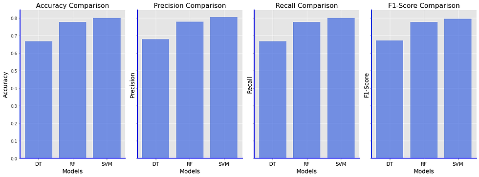
Comparison on Iris Flower Dataset

Now, let's compare the performance of these models on the Iris Flower dataset using a chart:

import matplotlib.pyplot as plt
import numpy as np
from sklearn.datasets import load_iris
from sklearn.model_selection import train_test_split
from sklearn.metrics import accuracy_score, precision_score, recall_score, f1_score
from sklearn.tree import DecisionTreeClassifier
from sklearn.ensemble import RandomForestClassifier
from sklearn.svm import SVC

# Load the Iris dataset
iris = load_iris()
X = iris.data[:, :2]
y = iris.target

# Split the data into train and test sets
X_train, X_test, y_train, y_test = train_test_split(X, y, test_size=0.3, random_state=42)

# Create and train the classification models
models = {
    "Decision Tree": DecisionTreeClassifier(),
    "Random Forest": RandomForestClassifier(),
    "Support Vector Machine": SVC()
}

# Initialize dictionaries to store evaluation metrics
metric_names = ['Accuracy', 'Precision', 'Recall', 'F1-Score']
metric_values = {metric: {} for metric in metric_names}

for name, model in models.items():
    model.fit(X_train, y_train)
    y_pred = model.predict(X_test)
    
    # Calculate evaluation metrics
    metric_values['Accuracy'][name] = accuracy_score(y_test, y_pred)
    metric_values['Precision'][name] = precision_score(y_test, y_pred, average='weighted')
    metric_values['Recall'][name] = recall_score(y_test, y_pred, average='weighted')
    metric_values['F1-Score'][name] = f1_score(y_test, y_pred, average='weighted')

# Create a grouped bar chart to compare metrics
models_names = models.keys()
abbreviated_names = ['DT', 'RF', 'SVM']

plt.figure(figsize=(16, 6))

for i, metric in enumerate(metric_names):
    plt.subplot(1, len(metric_names), i+1)
    bars = plt.bar(models_names, [metric_values[metric][name] for name in models_names], alpha=0.7)
    plt.xlabel("Models")  # Leave the x-axis label color as default (black)
    plt.ylabel(metric)  # Leave the y-axis label color as default (black)
    plt.title(f"{metric} Comparison")  # Leave the title color as default (black)
    
    # Customize x-axis labels with abbreviated names
    plt.gca().set_xticklabels(abbreviated_names)

plt.tight_layout()
plt.show()

Note that linear regression is not in the comparison due to the fact that is not a classification method and the only way to measure its accuracy will be with MSE.

In this blog post, we explored common supervised learning methods: Linear Regression, Decision Trees, Random Forests, and Support Vector Machines. Each of these methods has its strengths and weaknesses, making them suitable for different types of problems.

Linear Regression is straightforward but assumes linear relationships, while Decision Trees are versatile yet prone to overfitting. Random Forests mitigate overfitting and work well with high-dimensional data. Support Vector Machines are effective in high-dimensional spaces but require careful kernel and parameter selection.

In the next post, we will delve into unsupervised learning methods, expanding our understanding of machine learning techniques.

Stay tuned for our upcoming post on unsupervised learning!